Conduction velocity
See the tutorial for how to easily create a conduction velocity map.
Select [Conduction velocity map...] from the [analyze] menu.

On this dialog, a conduction velocity map can be created like below.
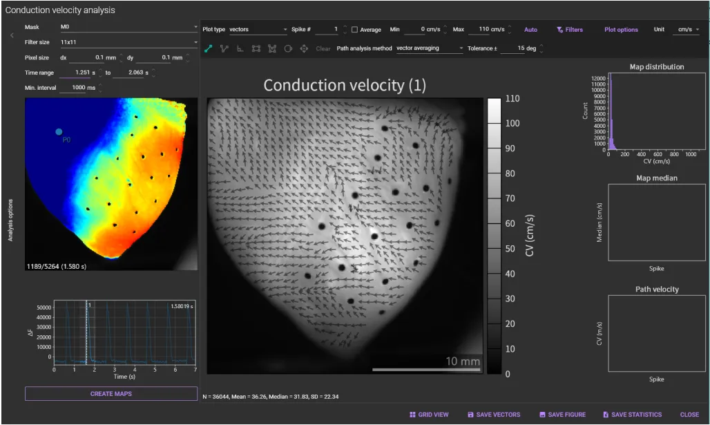

(1) Mask
Select the map creation area from “All pixels”, “Mx (mask)”, “Rx (region)”, "Cx (circle)".
(2) Filter size
Select the size of the spatial filter from None, 3x3, 5x5, 7x7, 9x9, 11x11, 13x13, 15x15. A background image does not change.
(3) Pixel size
You can specify the pixel size.
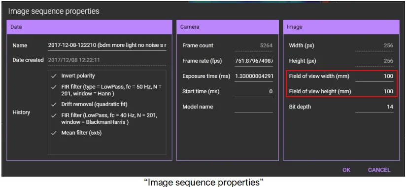
If “Field of view width (mm) / Field of view height (mm)” are already set on the “Image sequence properties” that opens when you right-click an image and select “Property”, pixel size is displayed in this area.
(4) Time range
Set a time range. Peaks outside this time range are ignored.
(5) Min. interval
Set a minimum time span between two peaks. This setting is used for automatic detection of peaks.
(6) Image display
Shows the same data as the main screen.
The following mouse operations are possible.
| Operation | Description |
|---|---|
| Scroll mouse wheel | Enlarge/reduce image size. |
| Mouse drag point | Light intensity change at the specified pixel is displayed in (7) . |
(7) Wave display
Display light intensity change in the pixel specified in (6) .
| Operation | Description |
|---|---|
| Scroll mouse wheel | Enlarge/reduce horizontal waveform size. |
| Mouse drag on waveform/Click on waveform | Move frame. |
| Hold “Ctrl” key and drag mouse pointer to right | Select time range of waveform. |
| Hold “Ctrl” key and drag mouse pointer to left | Deselect time range selection for waveform and select all ranges. |
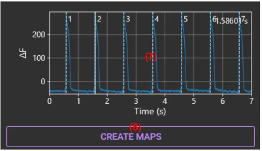
(8) CREATE MAPS
Create one map for each peak in the selected time range.
Click this button to automatically detect peaks and display peak numbers at the top of each waveform.


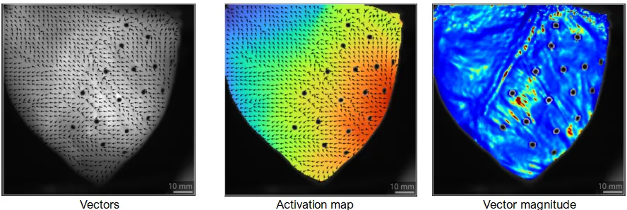
(9) Display
Select plot mode from “vectors”, “activation map” and “vector magnitude”.
(10) Spike
Select the number of peak (action potential or calcium transient) to display.
(11) Average
Click to create an average conduction velocity map for all peaks within the specified time range.
(12) Min
Specify the minimum value to be displayed in color.
(13) Max
Specify the maximum value to be displayed in color.
(14) Auto adjustment
Click to set min and max to optimal values.
(15) Filters
Specify a range of CV values. CVs with out-of-range values are not displayed.

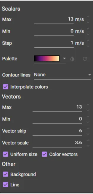
(16) Plot options
Change the CV display settings.
(17) Unit
Change the unit of CV display ("cm/s", "m/s", "mm/s").
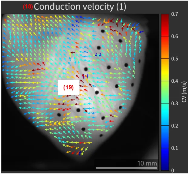
(18) Title and spike
The image title and spike # are automatically displayed.
(19) Map
A map created for each peak is shown here.
The following mouse operations are possible.
| Operation | Description |
|---|---|
| Mouse move over image | Coordinates, velocity and degrees are displayed on the top left of the map. |
| Left click | A straight line or polygonal line can be drawn on the image. Average conduction velocity on a line can be shown. To cancel line drawing and delete line, right click and select "Abort". To finish drawing the line, right click and select "End shape". 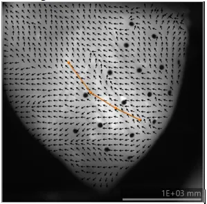 |

(20) Line
Draw a line on the image and calculate the average CV along the line. Left click to select the first point, then left click to select the last point.
(21) Polyline
Draw a polyline on the image and calculate the average CV along the polyline. Left click to select points other than the last, right click to select the last point and select [End shape] from the pop-up menu.
(22) Right angle
Draw a right angle on the image and calculate the average CV along the two lines. Left click to start drawing a right angle, then left click to end.
(23) Rectangle
Draw a rectangle on the image to specify the CV display area. Left click to select the left upper point of the rectangle, then left click to select the right bottom point of the rectangle.
(24) Polygon
Draw a polygon on the image to specify the CV display area. Left click to select points. The polygon is complete when the first and last points overlap.
(25) Circle
Draw a circle on the image to select the CV display area. Left click to start drawing a circle, then left click to end.
(26) Move shape
Move shape by mouse drag.
(27) Clear
Clear shapes on the image.
(28) Path analysis method
Select how to calculate CV on a line.
| end point time delta | CV is calculated without averaging. |
| vector averaging | CV is calculated with averaging. Calculates average CV in a rectangle within 5 pixels of the line, where CV direction is within the angle (specified by "Tolerance") of the selected line direction. |
(29) Tolerance
Specifies how many degrees of CV to the selected line direction should be included in the CV calculation.
(30) Map distribution
Shows relationship between CV values and the number of pixels.

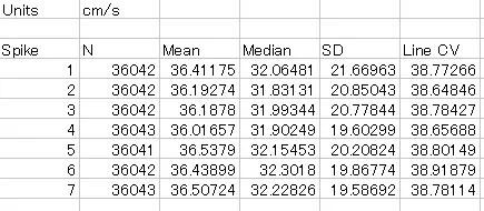
(31) Map median
Displays the median of the CV values for each spike (action potential or Ca2+ transient).

(32) Path velocity
Displays the average CV values for each spike (action potential or Ca2+ transient) along the path (line or polyline).


(33) GRID VIEW
Display multiple created maps in a grid. The number of columns can be changed with "Columns".
(34) SAVE VECTORS
Save vector data as the following formats.
| CSV (*.csv) | Comma separated 64-bit floating point values. See more details here |
| Apache Parquet (*.parquet) | Binary format that can be read by MATLAB, Python, etc. It is generally more efficient than CSV. See more details here. |
| DAT (*.dat) | Custom binary format used by BV workbench. The first 4 bytes indicates the data type. See more details here |
(35) SAVE FIGURE
Click to open “Figure editor”. See “Save image (figure editor)” for details.
(36) SAVE STATISTICS
Save statistical data in csv format.
(37) CLOSE
Close this dialog.