Analysis of Cardiac Mapping Data
Processing and analysis of cardiac mapping data using BV Workbench follows this paper.
Laughner JI, Ng FS, Sulkin MS, Arthur RM, Efimov IR.
Processing and analysis of cardiac optical mapping data obtained with potentiometric dyes.
Am J Physiol Heart Circ Physiol. 2012 Oct 1;303(7):H753-65.
If you want to know the basic usage of BV Workbench, please refer to "Basic operation".
1. Data processing
1-0. Processings according to data
These processings ("Invert polarity", "Crop" and "Create subset") are not always necessary. Whether to use these processings depends on data.
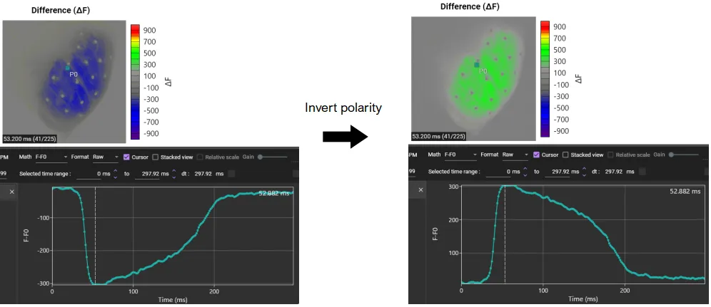
Invert polarity (for negative delta F signals)
Select [Filter toolbox...] from [Process] menu.
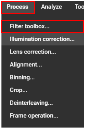
Select [Invert] from the list on the left. After confirming that "Invert" is displayed in the central list, click [Apply].

![]()
Crop (when sample size is smaller compared to the field of view size)
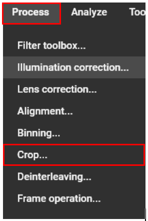
Click [Process]-[Crop] to open the following dialog.
On this dialog, you can crop a part of an image. Drag mouse cursor from upper left to lower right on an image, or enter coordinates, width, and height to specify range.
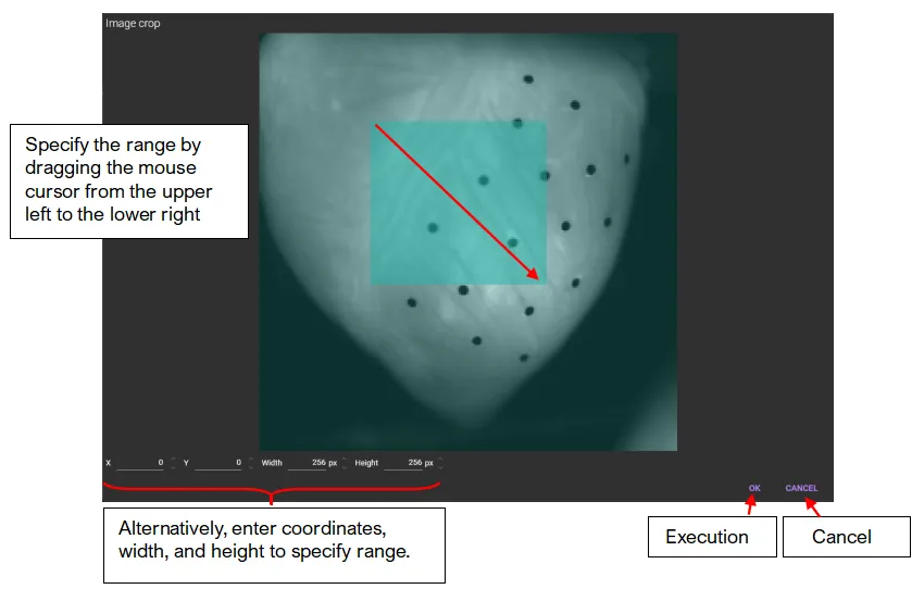
Cropped image is displayed. This process can be undone with the “Undo” button.

Create subset (if time range needs to be limited)
You can cut out only some time range of data and open/save it as new data.
Hold down “Ctrl” key and drag mouse from left to right on waveform to specify time range.
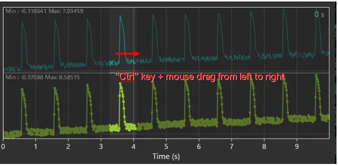
Select [Create subset...] from [File] menu.

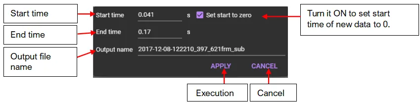
Enter start time, end time, output data name, and click "APPLY" to display as separate data.
Data displayed as separate data is not saved. Save it by clicking [Save dataset].
1. Data masking
Specify the data analysis area. There are two ways, "ROI" and "Add mask".
It is recommended to use "ROI" to specify the region when difference in light intensity between sample and out-of-sample is not obvious. ROI types include rectangle, polygon, and circle.
If difference in light intensity between sample and out-of-sample is obvious, you can also specify the region with "Add mask".
1-1. ROI (Polygon)
See ROI(Polygon) for details.
With "Add polygon" ![]() selected, click on image and specify polygon. A polygon is completed when start point and end point are specified to be the same.
selected, click on image and specify polygon. A polygon is completed when start point and end point are specified to be the same.
The specified polygon becomes ROI (Region of Interest) and is used for target range of various data analysis.
1-2. Add mask
See "Mask" for details.
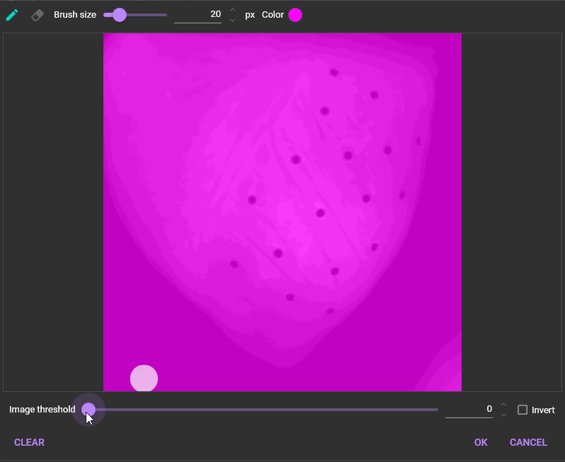
“Mask” is an area to be used for data analysis by specifying a threshold for image brightness.
To use “Mask”, click ![]() and select [Add mask].
and select [Add mask].

The following dialog will appear. Select the threshold for image intensity to specify the data analysis range. The data analysis range is displayed in pink.
2. Spatial filter
Remove noise.
See "2D Convolution filter (Mean/Gaussian)", "Median filter" for details.
Select [Filter toolbox...] from [Process] menu.
Select either "2D Convolution filer" or "Median filter" and set parameters.
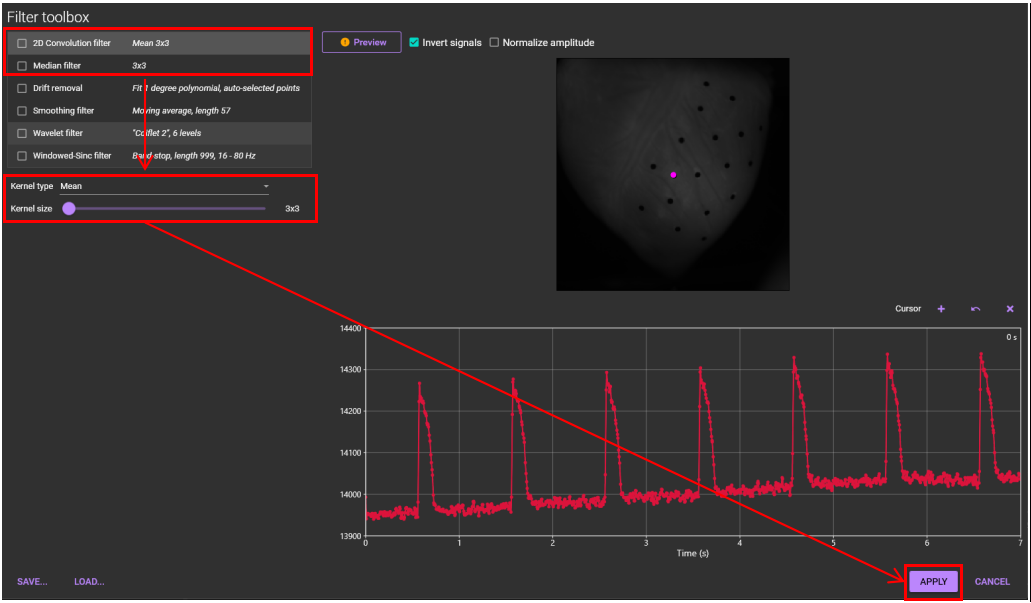
Click [APPLY], or you can select multiple filters before clicking [APPLY].
3. Temporal filter
Remove noise.
Select [Filter toolbox...] from [Process] menu.
Select "Smoothing filter" or "Wavelet filter" or "Windowed-Sinc filter" and set parameters.
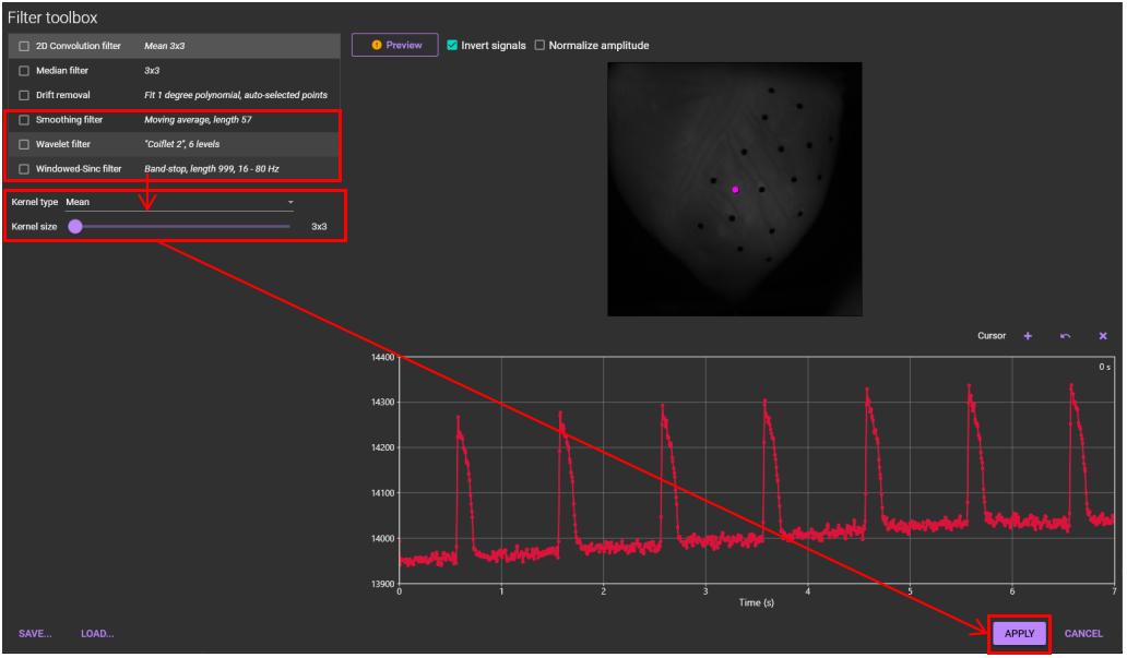
Click "APPLY", or you can select multiple filters before clicking "APPLY".
4. Drift removal
Remove baseline drift.
See "Drift removal" for details.
Select [Filter toolbox...] from [Process] menu.
Select "Drift removal" and set parameters.
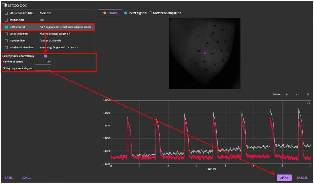
Click [APPLY]. Baseline drift is corrected.

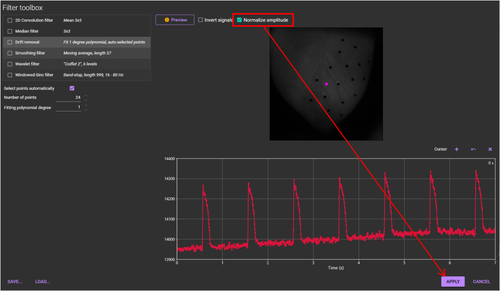
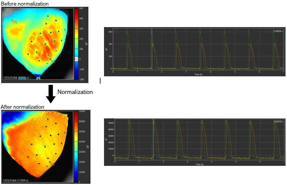
5. Normalization
Data is normalized.
See "Normalization" for details.
Select [Filter toolbox...] from [Process] menu.
Select [Normalize amplitude] in the list on the "Filter toolbox". Then, click [APPLY].
B. Data analysis
1. Activation map
Select [Time domain analysis...] from [Analyze] menu.

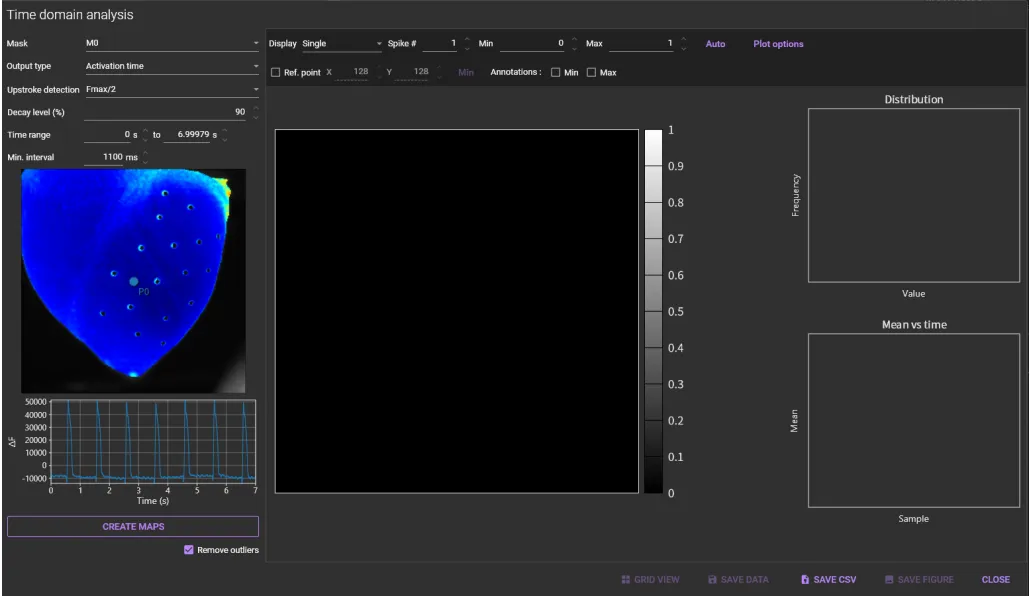
Select a mask name (ROI name) from the [Mask] list box.
Select "Activation time" from the [Output type] list box.
Select activation time ("Fmax/2" or "Fmax" or "max(dF/dt)") from the [Upstroke detection] list box.

Select a time range on waveform by holding down the "Ctrl" key and drag the mouse pointer to right.
(This is not necessary if you want to use the entire time range)
Click [CREATE MAPS].
![]()
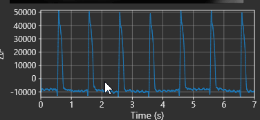
Action potential (or Ca2+ transient) peaks are automatically detected and numbered above each peak.

If some peaks are not detected automatically, adjust the [Min.interval] (minimum time span between two peaks) and click [CREATE MAPS] again.

All selected peaks are detected as shown in the image below.

"Activation time map" is displayed. Click [Auto] to set the appropriate time range and change the map display.
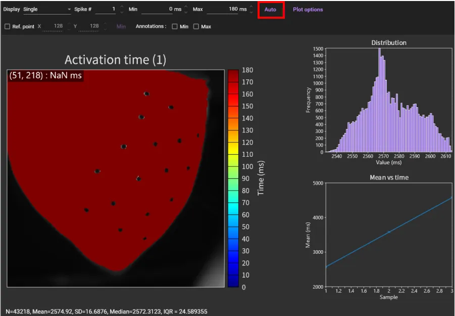
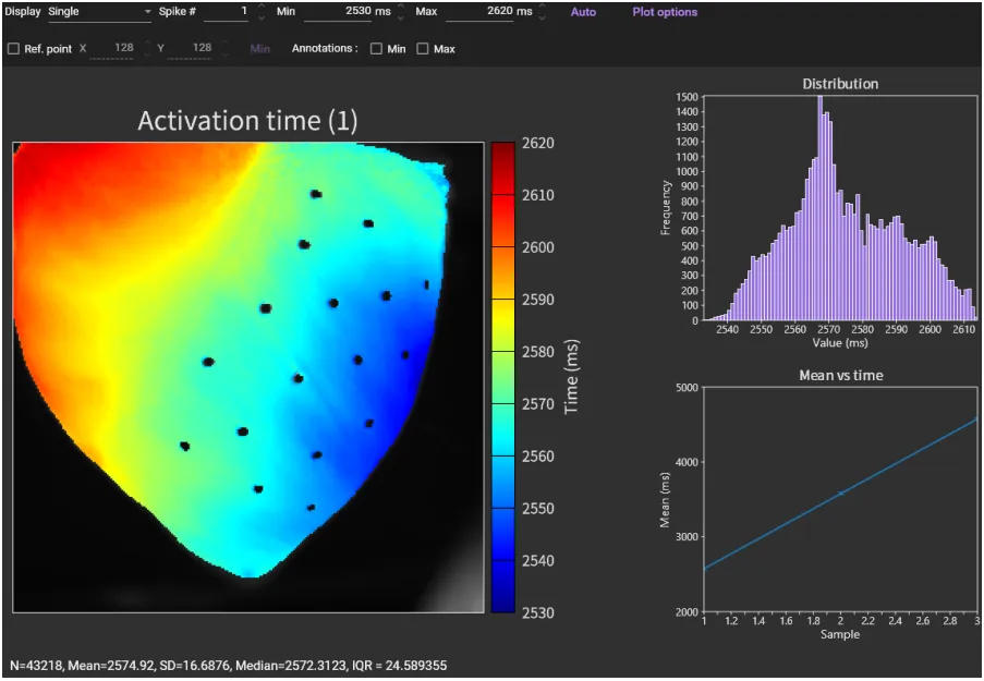
Click [Spike #] to display the map corresponding to the peak number.

However, by default, the map is created with the beginning of the selected time range set to 0msec, so the color scale is different for each map.
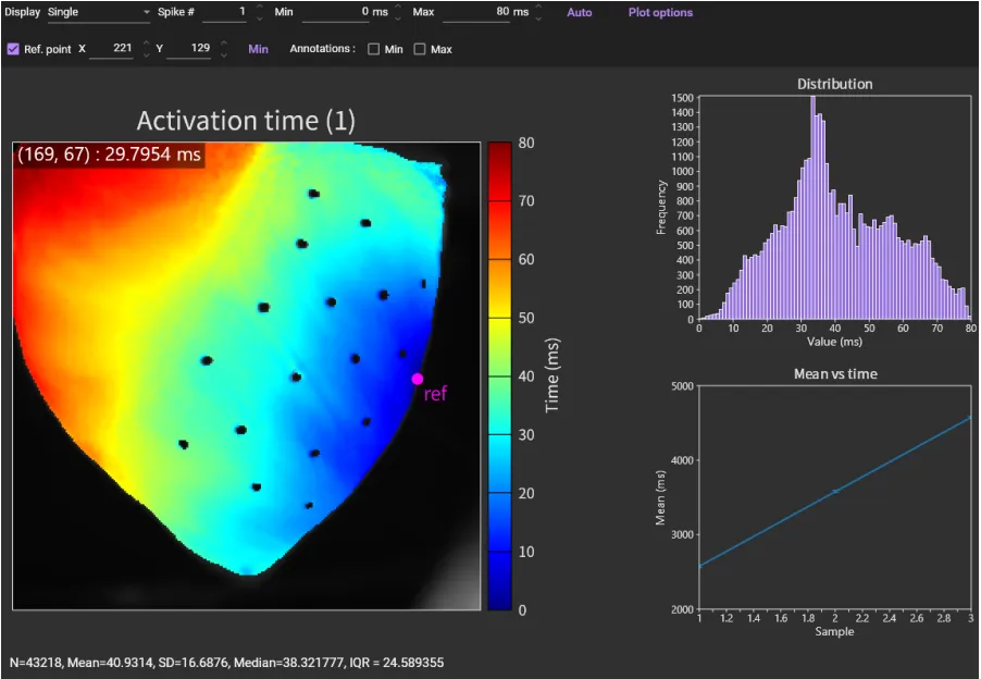
If you have created multiple maps using the same color scale, select [Ref. point]. A pink dot will appear on the image, so drag that dot to the pixel where the activation time is 0msec. Or click [Min] to automatically move the pink dot to the minimum value pixel.
![]()
Then, click [Auto] again. Click [Spike #] to see other spikes (action potential/ca2+ transient).
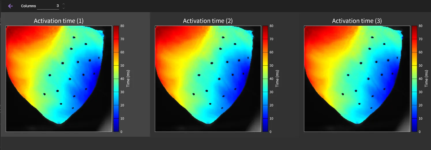
Click [GRID VIEW] to display all maps corresponding to each peak.

2. Conduction velocity map
Select [Conduction velocity map...] from [Analyze] menu.

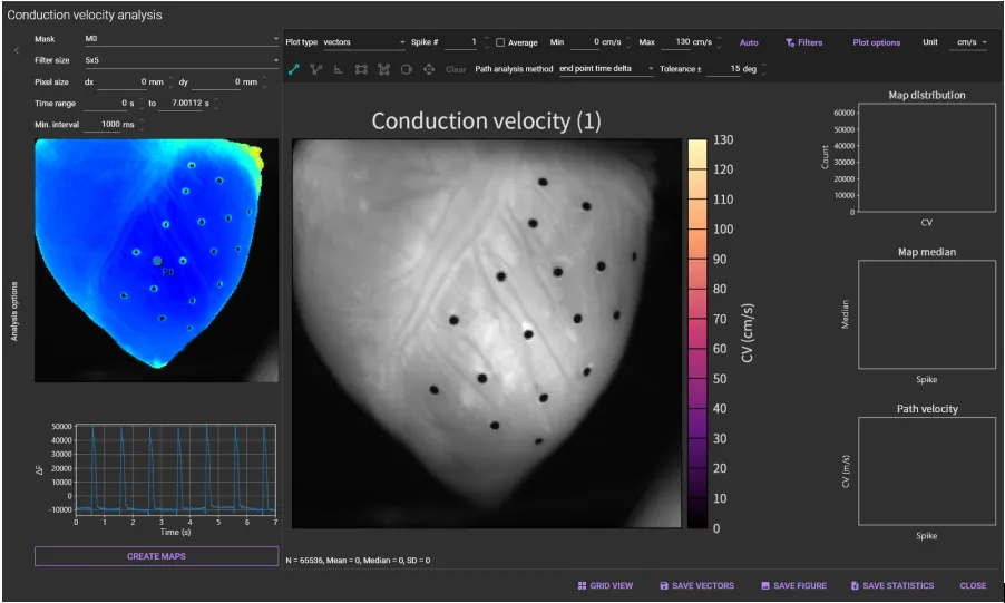
Select a mask name (ROI name) from the [Mask] list box.
Select [Filter size] (size of the convolution filter applied to the activation time values) from the [Filter size] list box.
Set vertical/horizontal pixel size.

Select a time range on waveform by holding down the "Ctrl" key and drag the mouse pointer to right.
(This is not necessary if you want to use the entire time range)
Click [CREATE MAPS].
![]()
Action potential (or Ca2+ transient) peaks are automatically detected and numbered above each peak.
If some peaks are not detected automatically, adjust the [Min.interval] (minimum time span between two peaks) and click [CREATE MAPS] again.

All selected peaks are detected as shown in the image below.
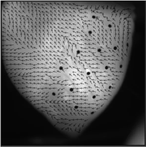
"Conduction velocity map" is displayed.
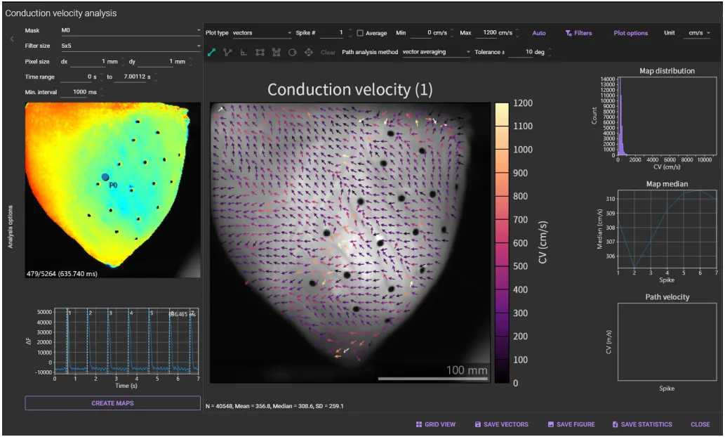
If conduction velocities are not displayed on the image, click [Filters] and adjust the filter range.

Click [Auto] to set the appropriate value range and change the map display.
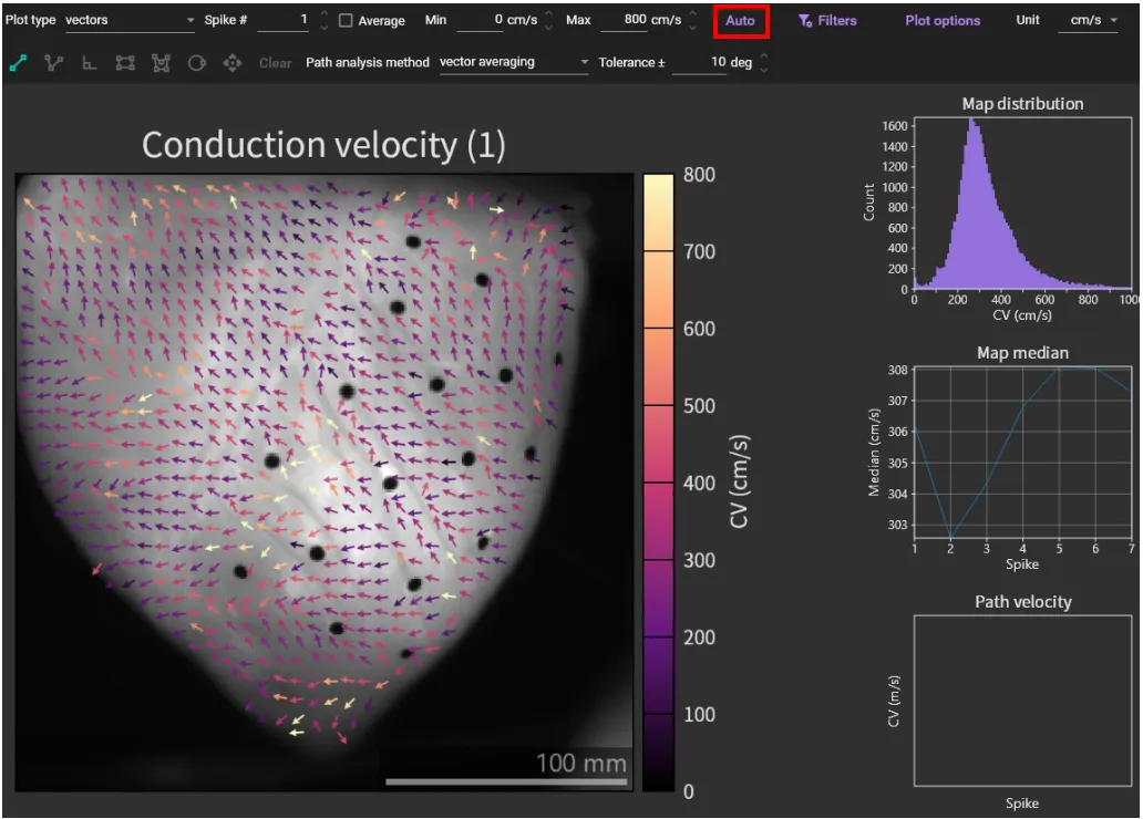
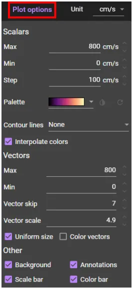
Click [Plot options] and you can change the display settings of conduction velocity.
3. Conduction velocity on line
Click [Line] to draw a straight line on the image.

Select start and end points by left-click on the starting point of the direction, then left-click on the ending point.
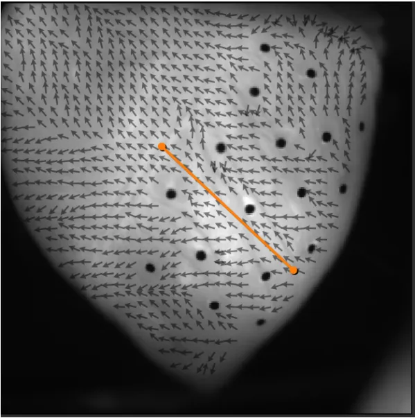
If you want to clear and redraw the line, click [Clear].

If "vector averaging" is selected from [Path analysis method] list box and "15deg" is set in the [Tolerance ±], it calculates average CV in a rectangle within 5 pixels of the line and with CV direction within 15deg of the selected line direction.
![]()
The CV information on the specified line is displayed at the bottom right of the window.

Click [SAVE STATISTICS] to output values to a CSV file.

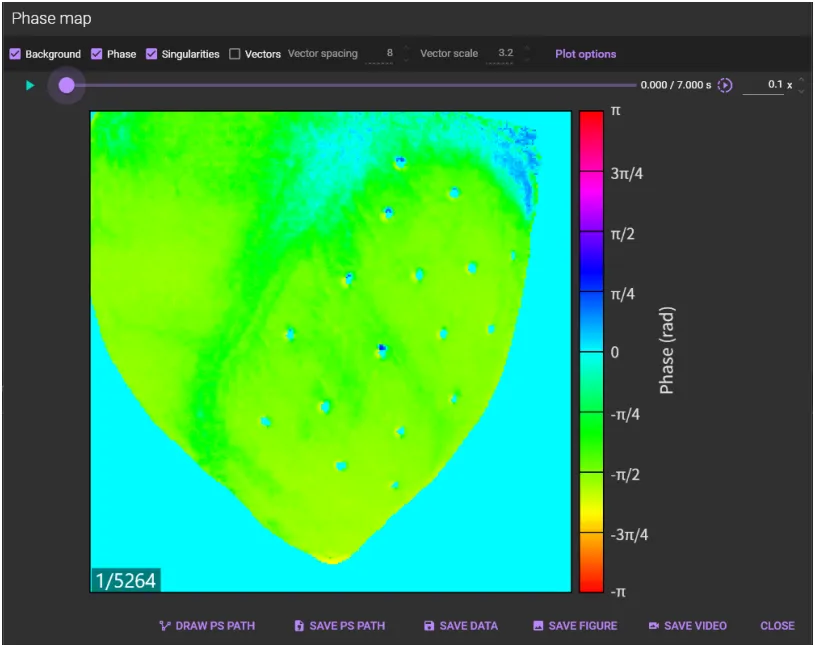
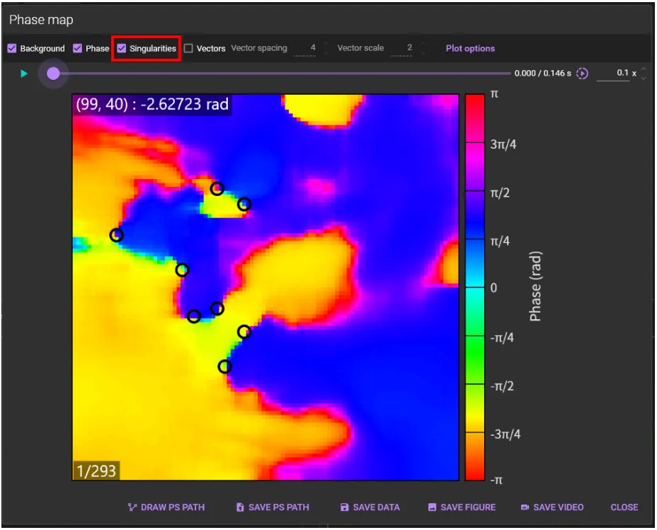
4. Phase map
Hold down “Ctrl” key and drag mouse from left to right on waveform to specify time range.
Select [Phase map...] from [Analyze] menu.

A phase map is displayed.
When [Singularities] is selected, phase singularities are displayed as black circles.
5. Save image
If you click [SAVE FIGURES] on each dialog, the dialog for saving figure will be displayed and you can save the high resolution figure.

A "Figure editor" will appear.
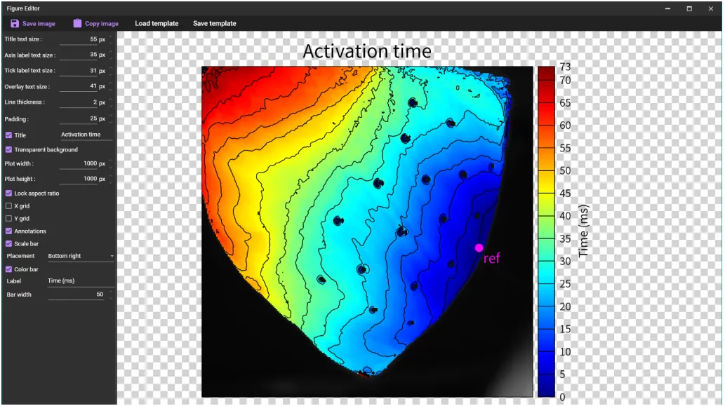
You can change figure settings. In particular, you can change the number of pixels with [Plot width] and [Plot height].

You can save the figure in "webp or "SVG" format by clicking [Save image].
