Cardiac Optical Mapping Data Analysis for hiPSC-CMs Stained with Voltage-Sensitive Dye


- Sample
- Human induced pluripotent stem cell-derived cardiomyocytes (hiPSC-CMs)
- Fluorescence Dye
- Voltage sensitive dye (FluoVolt)
- Imaging System
- MiCAM05-Ultima
- Pixels
- 100x100
- Frame Rate
- 200fps (5.0msec/frame)
- Provided by
-
Dr. Hee Jae Jang, Dr. Vladislav Leonov and Dr. Alexey
Glukhov
University of Wisconsin-Madison
0. Overview
This page explains how to analyze cultured cardiomyocyte data and create maps such as activation map and CV map by using BV Workbench.
1. Start BV Workbench
Start BV Workbench by double-clicking the icon on the desktop or clicking the icon in the Windows Start menu.

BV Workbench starts up.

2. Open dataset / Import data
2-1. Load data
To import a single raw/gsd/tiff file, click the [Import]. To open dataset, click [Open].

If you click [Import], select a single data file (raw, tif, gsd, rsh) and click [Open].

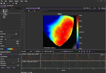
A preview of the data is displayed. Click [View waveform] to display waveform.

Click [OK] to load data.

2-2. Change color map
If you want to change the color map (pseudo color), Select data name in the tree at the upper left of the screen.
Click [Palette] and select a new color map. In most cases, a gray colormap is chosen for background image.

Changed to black and white color map.

Click [A] to automatically adjust gain of background image.

To save color map settings, click [Set current settings as default] button.

Click on an image to display waveform (intensity change) of clicked point.

3. Change display mode and color map
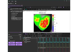
Next, change color map of ΔF image. Select ΔF from the [Mode] list.

Click [Palette] and select a new color map.

Changed to different color map. Click [A] to automatically adjust gain of ΔF image.

To specify/change baseline (F0), click on waveform to select frame you want to use as baseline.
Select [Set current frame as baseline (F0)] from the three-dot menu.

The baseline will change so that the selected frame is the 0 point.

4. Data masking / ROI
Specify ROI to be used for data analysis.
Changing mode to "F" will display a black and white background image.

Select [Add polygon] to set ROI.

Click on the image to enclose the sample and specify the ROI.

Click so that the start and end points are the same.

Set the display mode to "ΔF" and the display area to "ROI".

You can see the brightness changes displayed in pseudocolor only in the selected range.

5. Filter / Data processing
Select [Filter toolbox...] from [Process] menu.

[Filter toolbox] is displayed.

Here we use three types of filters.
| Filters | Description |
|---|---|
| 2D Convolution filter | Spatial filters such as Mean filter and Gaussian filter |
| Drift removal | Filter to remove baseline fluctuations and drifts |
| Windowed-Sinc filter | Frequency filters such as low-pass filter, high-pass filter, band-pass filter |
2D Convolution filter
After checking the [2D Convolution filter] box, select "Mean" or "Gaussian" for [Kernel type] and specify the kernel size. The higher the kernel size, the stronger the spatial filter will be.

Click [Preview] to see the results after filtering.

Drift removal
Turn on the [Drift removal] checkbox and click on [Drift removal] to display the parameter settings below. Normally the optimal values are set automatically, but you can change them to any values.

Windowed-Sinc filter
Turn on the [Windowed-Sinc filter] checkbox and click [Windowed-Sinc filter] to display the parameter settings below. Normally, the optimum value is set automatically, but you can change it to any number.
To remove high-frequency flickering noise, select "Filter type=Low-pass".

Once you have finished setting up, click the [Apply] button.

The filtered data is displayed. Click [A] to automatically adjust gain of image.

When filtering is performed, baseline of waveform may move to negative side. In that case, you can set baseline to 0 by selecting "Set baseline from minimum" or "Set current frame as baseline (F0)" from the three-point menu.


Play the video and check the signal propagation.

6. Activation time map
Select [Time domain analysis] from the [Analyze] menu.

[Time domain analysis] screen is displayed.

Select "Output type=Activation time". Set other parameters accordingly.

Click [Create maps] and each peak will be automatically recognized and numbered.

If the automatic peak detection does not work, change the [Min. interval] and click [Create maps] again. "Min. interval" is the minimum time span between two peaks.

Click [A] to set optimal time interval.

By default, start time of activation time is start time of data. To set start time for each activation map, click "Ref. Point (reference point)".
A pink dot will appear on an image indicating the reference point. When you click "Min", the pink dot will automatically move to point where activation time is minimum. To set it manually, drag the pink dot.

Click [A] to set optimal time interval.

To set contour lines, select [Black] from [Plot options]-[Contour lines].

To change interval of contour lines, click [Edit color map] and change [Step]. Then, click [Apply].


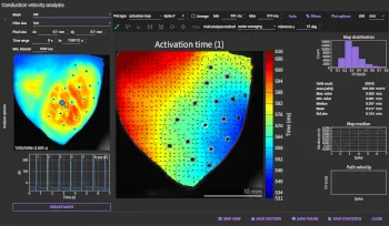
7. Conduction velocity map
From the [Analyze] menu, select [Conduction velocity map...].

[Conduction velocity analysis] screen is displayed.

Enter size of one pixel of camera in mm.

Click [Create maps] to display vectors.

If vectors are not displayed, turn off [Vector options]-[Filer by value].

Adjust [Skip] and [Scale] to adjust density and length of vectors.


Click the "Tile" icon. CV maps will be displayed in tiles.


You can save CV map as a high-resolution image by clicking [Save figure].

Product information
- Analysis Software for Optical Mapping and Calcium Imaging
- BV Workbench
BV Workbench Ver.4 is the latest version of data analysis
software developed for optical mapping and calcium imaging
of the brain and heart.
In addition to data files
acquired with Brainvision's MiCAM imaging system, it is also
possible to open 16-bit TIFF files acquired with cameras and
imaging systems from other companies.
- High Speed Imaging System
- MiCAM03-N256
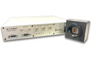
MiCAM03-N256 is a high-speed imaging system that captures and visualizes small changes in fluorescence intensity from biological samples stained with fluorescent probes, such as voltage sensitive dyes and calcium dyes.
- Spatial Resolution :
-
128x128 - 256x256 pixles
(32x32 pixels - 256x256 pixles with option) - Maximum Frame Rate :
- 1,000fps
(20,000 fps available with option) - Up to 2 camera heads can be used with completely synchronization.