From Raw Data to Publication-Quality Figures!
Advanced S/N Ratio Enhancement and Noise Reduction Techniques in BV Workbench

The Critical Importance of Signal-to-Noise Ratio (S/N) in Optical Mapping Data Analysis

Optical mapping, a technique for visualizing action potentials and calcium dynamics in the brain and heart, is a cornerstone of fundamental biomedical research.

This method utilizes voltage-sensitive dyes like Di-4-ANEPPS and FluoVolt, calcium-sensitive indicators such as Fluo-4 and Cal520, as well as fluorescent proteins including GECIs, GEVIs (including FRET-based sensors), and intrinsic signals from hemoglobin or flavin fluorescence proteins.

The fluorescence signals obtained from these measurements are exceedingly faint and inevitably contaminated by noise from the optical system, biological tissue, and random electronic noise.

Therefore, maximizing the signal-to-noise ratio (S/N ratio) is essential for accurately extracting the true signal from the raw data and ensuring the reliability of the findings.

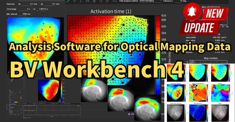
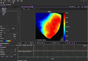
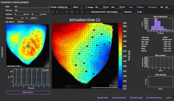
BV Workbench, the latest version of our optical mapping data analysis software, supports the import of 16-bit TIFF files from Brainvision's MiCAM imaging systems and other manufacturers' camera systems. It is engineered to rapidly generate high-precision output data suitable for scientific publications.

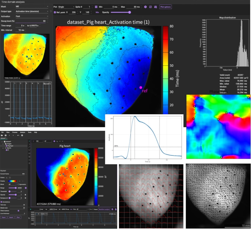
Screen images of BV Workbench

This article provides a detailed guide to the practical techniques for improving the S/N ratio and obtaining high-precision data (e.g., Activation maps, APD maps, Conduction velocity maps) by focusing on the diverse array of noise reduction filters and data correction functionalities integrated into BV Workbench Ver. 4.6.7.

1. Basic Filters for Spatial Noise Removal

Since optical mapping data is treated as a time series of images, the first step in enhancing the S/N ratio is to remove spatial noise (e.g., random noise, granular noise) contained within individual frames.

These spatial filters can be selected and applied from the "Filter toolbox" in BV Workbench.

Filter toolbox dialog

1-1. 2D Convolution filter (Mean/Gaussian)

The 2D convolution filter is a standard method for smoothing images and removing noise. Convolution is a process that modifies an image by using a small matrix called a kernel (or convolution matrix, mask) to calculate a weighted sum of each pixel and its neighbors.

1-1-1. Mean filter

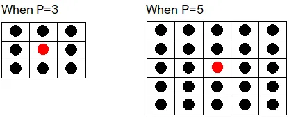
The Mean filter smooths an image and reduces noise. The user specifies the "Kernel size."

For instance, a kernel size of 3 sets the central pixel to the average of the surrounding 9 pixels (3x3), while a size of 5 uses the average of 25 pixels (5x5). A larger value applies a stronger filtering effect.

1-1-2. Gaussian filter

The Gaussian filter also smooths images and reduces noise. It is particularly effective at reducing noise while relatively preserving sharp edges in the image.

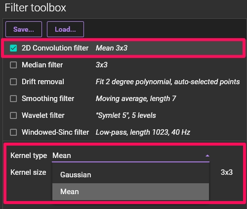
Operating Steps
1. Select "2D Convolution filter" in the "Filter toolbox" panel.
2. Choose "Mean" or "Gaussian" from the "Kernel type" dropdown menu.
3. Specify the "Kernel size." A higher value results in a stronger filter application.
4. Confirm the effect using the "Preview" button, then click [APPLY].

1-2. Median filter

The Median filter is a non-linear digital filtering technique used for smoothing images and reducing noise.

A key feature of this filter is that it sorts the values of the pixels in the vicinity (window/kernel) of a target pixel and replaces the target pixel's value with the median value. This method is highly effective at removing abrupt signal changes, such as spike noise or salt-and-pepper noise, while better preserving edges compared to mean filters. It has been shown to be far superior to moving average filters for dealing with impulse noise.

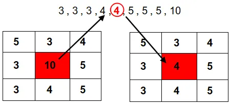
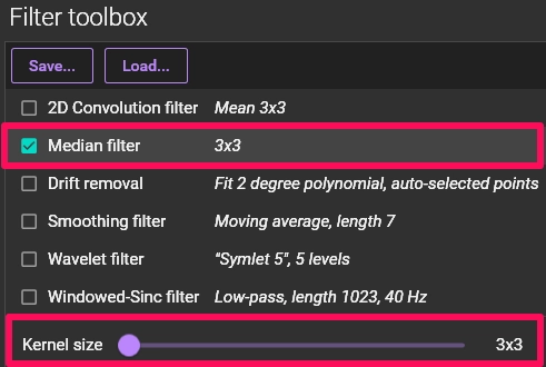
Operating Steps
1. Select "Median filter" in the "Filter toolbox" panel.
2. Specify the "Kernel size." A higher value results in a stronger filter application.
3. Confirm the effect using the "Preview" button, then click [APPLY].

2. Advanced Filters for Temporal Noise (Waveform) Removal

In optical mapping analysis, removing noise from the time-series data (waveform) of each pixel is directly linked to the accuracy of APD maps and conduction velocity maps. BV Workbench offers various temporal filtering options.

2-1. Smoothing filter (Moving average/Savitzky-Golay)

This filter is used to smooth signals (waveforms) and remove noise. Users can select either the "Moving average filter" or the "Savitzky-Golay filter" as the method.

2-1-1. Moving average filter

The moving average is a statistical technique that smooths out short-term fluctuations and highlights long-term trends or cycles by calculating a series of averages of different fixed-size subsets of the full data set.

From a signal processing perspective, the moving average is a type of low-pass FIR (Finite Impulse Response) filter, also referred to as a "boxcar filter."

2-1-2. Savitzky-Golay filter

The Savitzky-Golay filter is a digital filter designed to smooth a set of digital data points to increase the precision of the data without distorting the signal tendency.

This is achieved by fitting successive sub-sets of adjacent data points with a low-degree polynomial using the method of linear least squares.

When the data points are equally spaced, an analytical solution for the set of "convolution coefficients" can be found, which can be used to calculate the smoothed signal estimate. The moving average filter can be considered the simplest case of a Savitzky-Golay filter, where the data is fitted with a polynomial of degree 0 or 1.

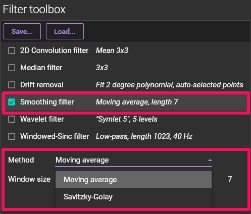
Operating Steps
1. Select "Smoothing filter" in the "Filter toolbox" panel.
2. Choose "Moving average" or "Savitzky-Golay" from the "Method" dropdown menu.
3. Specify the "Window size." A higher value applies the filter more strongly. As you change the value, the filtered waveform is automatically displayed in red, allowing for real-time confirmation of the effect.
4. Click [APPLY] to apply the filter.

2-2. Drift removal: Correcting Baseline Fluctuations

This function corrects for the rise or fall (drift) of the waveform baseline caused by factors such as photobleaching of fluorescent dyes or slight variations in light source intensity.

Since drift can introduce systematic errors into the analysis results, its removal is essential.

This function works by fitting a polynomial function to the signal's baseline and then subtracting it.

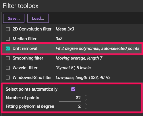
Operating Steps
1. Select "Drift removal" in the "Filter toolbox" panel.
2. Turn on "Select points automatically" and set the "Number of points" and "Fitting polynomial degree."
3. As you change the values, the waveform after drift removal is automatically displayed in red, allowing for immediate confirmation of the correction result.
4. Click [APPLY] to apply. An option to manually set fitting points is also available.

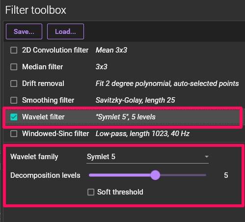
2-3. Wavelet filter

The Wavelet filter is an advanced technique used for signal denoising. It is based on the Discrete Wavelet Transform (DWT). A key advantage of the DWT, compared to the Fourier transform, is its ability to capture both frequency information and time/location information (temporal resolution).

The wavelet transform is computed by passing the signal through a series of filters, resulting in detail coefficients from a high-pass filter and approximation coefficients from a low-pass filter. It has a wide range of applications, including image processing, data compression, and noise removal.

In BV Workbench, you can select the most suitable wavelet family for noise reduction (e.g., Harr, Coiflet, Daubechies, Symlet) to reduce noise.

2-4. Windowed-Sinc filter

The Windowed-Sinc filter is used to remove noise from temporal waveforms.

The Sinc filter is known as an ideal low-pass filter. It removes all frequency components above a given cutoff frequency without attenuating lower frequencies.

However, the ideal Sinc filter is non-causal and has an infinite impulse response, making it impractical for real-world applications. Therefore, it is approximated by applying a window function to the ideal Sinc filter kernel, effectively truncating it.

In BV Workbench, the Windowed-Sinc filter can be used to perform low-pass, high-pass, band-pass, or band-stop filtering.

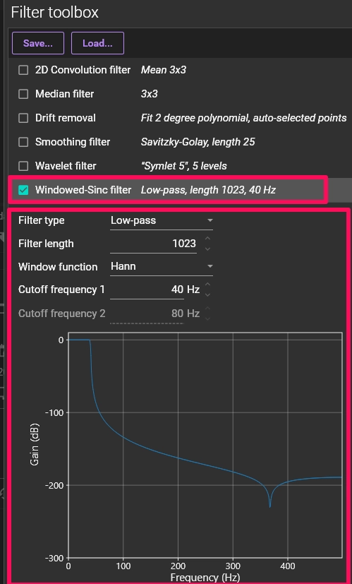
Operating Steps
1. Select "Windowed-Sinc filter" in the "Filter toolbox" panel.
2. Set the filter parameters.
3. As you change the values, the filtered waveform is automatically displayed in red, allowing you to adjust settings while confirming the result.
4. Click [APPLY] to apply.

3. Techniques for Improving S/N Ratio through Data Integration

In addition to applying noise reduction filters, data can be combined and manipulated to radically improve the signal-to-noise ratio based on statistical principles.

3-1. Binning: Pixel integration for improved S/N ratio

The Binning function is used to combine multiple adjacent pixels in an image into a single pixel.

This process reduces the number of pixels in the image, but in turn, improves the S/N ratio. This is because random noise tends to cancel itself out, while the signal adds up coherently. You can choose between "Sum" or "Average" as the calculation method when combining pixels.

Binning

Operating Steps
1. Select [Process] - [Binning] to open the dialog box.
2. Choose the calculation method ("Mode") and set the binning size ("Size").

3-2. Average datasets: Removing Inter-Trial Noise

You can calculate the average of datasets obtained from multiple trials to create a new dataset. Notably, even if noise temporarily contaminates one acquisition, it is possible to exclude the noisy data and perform offline averaging using the other datasets. This enables highly reliable average waveform and map analysis.

Operating Steps
1. Click [Tools] - [Average datasets...] to open the dialog box.

3-3. Alignment: Accurate Superimposition of Multiple Data

When performing subtraction or division between identical pixels of two datasets, even slight movements or shifts of the sample (heart or brain) can compromise analysis accuracy.

The Alignment function is used to scale, rotate, and translate image data. If two or more data exist within the same file, this function can be used to finely superimpose the two datasets. This is a crucial preprocessing step for ratio calculation.

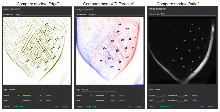
Operating Steps
1. Select [Process] - [Alignment...] to open the dialog box.
2. Set the scaling, rotation, and translation in the dialog box.

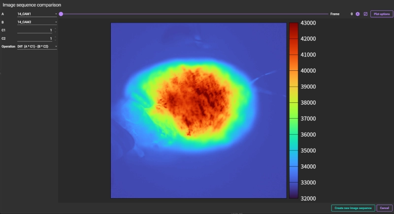
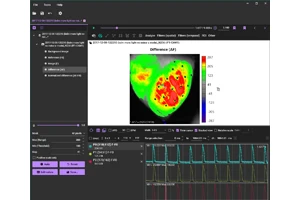
3-4. Frame operation: Arithmetic Operations Between Datasets

If a single data file contains multiple datasets (image sequences), the Frame operation function allows you to perform arithmetic operations (addition, subtraction, multiplication, division) between two of them.

The calculation includes all frames within the datasets. This can be applied to calculations for ratiometric imaging and for precise background subtraction.

3-5. Other Data Manipulation and Preprocessing Functions

Crop

A function to cut out a part of an image. You can specify the region by dragging the mouse or entering coordinates to reduce unnecessary areas.

Image crop

Time slice (Create subset)

Allows you to extract a specific time range from the data and open or save it as a new dataset. Specify the time range by holding the Ctrl key and dragging the mouse on the waveform, then set the start time, end time, and output data name.

Time slice (create subset)

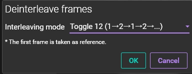
Deinterleave frames

For dual-wavelength excitation/single-wavelength emission imaging like with GCaMP or Fura-2, frames acquired at two different wavelengths are interleaved.

This function separates the frames by wavelength from one dataset, dividing it into two independent datasets.

4. Correction and Optimization Functions to Maximize Data Precision

In addition to noise removal, optimizing the tonal range and amplitude characteristics of the acquired data can enhance the precision and visibility of the results (level correction functions).

4-1. Dynamic range optimization (DRO)

Due to factors such as sample staining conditions, optical system issues, or sampling rate settings, images may be captured that are dark, utilizing only a fraction of the 16-bit dynamic range (0-65535). In such situations, the signal amplitude is very small and vulnerable to quantization error.

The DRO function optimizes the brightness value of each pixel, calculating and applying a gain and offset so that the minimum value becomes 0 and the maximum value becomes 65535, thereby scaling the data to use the entire 16-bit dynamic range. This corrects dark images, making them brighter and expanding the dynamic range.

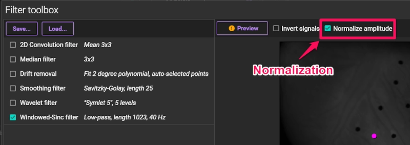
4-2. Normalization (Normalize amplitude)

Normalization corrects for differences in the amplitude of light intensity values among pixels, calculating so that the brightness values of all pixels have the same amplitude (0-65,535).

For example, even in a uniform tissue sample like an isolated heart, external factors such as uneven excitation light, inconsistent staining, or differences in tissue thickness can cause fluorescence intensity to vary by location.

Using Normalization removes the influence of these external factors, making the signal intensity (waveform) of all pixels uniform in amplitude, similar to what would be recorded with an electrode.

Algorithm of Normalization
1. For each pixel, check all frames to find the maximum and minimum values.
2. Calculate the gain and offset required to make the minimum value 0 and the maximum value 65535.
3. Apply the calculated gain and offset to all frames for that pixel.

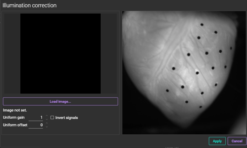
4-3. Illumination correction

This function corrects for vignetting (darkening of image corners) caused by the optical system and unevenness in excitation light intensity in software, making the background brightness of the screen nearly uniform.

To perform this correction, you need to load a uniform, non-saturated background image, such as one of a blank piece of paper. The process multiplies each pixel by a gain factor to bring the saturation of all pixels close to 100%.

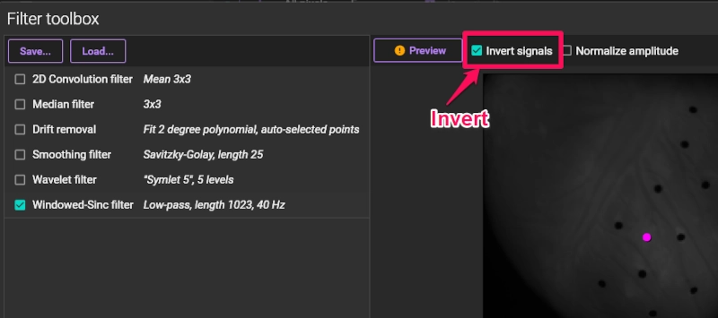
4-4. Invert

This function inverts the polarity of the signal (the polarity of the F-F(0) change). The light intensity values of the background image (baseline) are maintained. It can be executed by selecting "Invert signals" from the Filter toolbox.

5. Accelerating Analysis Workflows with Filter Batch Processing (Filter toolbox)

Data analysis for publication often involves repeating multiple filtering processes and cycles of trial and error. The "Filter toolbox" feature in BV Workbench significantly streamlines this process.

The Filter toolbox dialog allows users to select multiple filters from a list (e.g., 2D Convolution filter, Drift removal, Smoothing filter) and have them executed sequentially in a batch process with specified settings. The filters are designed to be processed in an optimal order.

5-1. Real-time Result Confirmation and Optimization

The Filter toolbox includes the following features

* Preview image: Displays an image preview of the filtering result.
* Waveform display: Shows the waveform of a selected point, allowing real-time confirmation of how the waveform changes after filtering.

Preview image and waveform display

These preview functions enable researchers to intuitively evaluate the effects of noise reduction and the impact on the signal while adjusting parameters.

5-2. Automatic Optimal Value Setting and Configuration Saving

Some features in BV Workbench are designed to automatically set optimal values without user input. This allows even users with limited analysis experience to quickly start high-precision data processing.

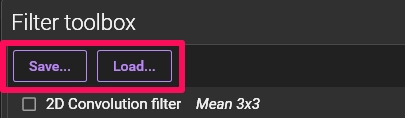
Furthermore, a series of filter settings can be saved to a file (SAVE) and loaded from a previously saved file (LOAD), ensuring consistency and reproducibility in the analysis.

Conclusion: A Data Analysis Environment Directly Leading to Scientific Publications

BV Workbench is a versatile analysis software suitable for a wide range of cardiac and neural imaging applications, including Langendorff-perfused hearts, brain slices, and cultured neurons.

By leveraging the software's powerful S/N enhancement filters—spatial noise removal with Mean/Gaussian and Median filters; temporal noise removal with Moving average, Savitzky-Golay, Wavelet, and Windowed-Sinc filters—along with data integration techniques like Binning and Average datasets, and advanced data correction functions such as DRO and Normalization, researchers can rapidly generate the highest quality, publication-level data from their raw recordings.

The final analysis results can be exported as a variety of specialized map images, such as Activation maps, APD maps, and Conduction velocity maps. The ability to export in high resolution as PNG format (ideal for high-definition printing) or SVG format (vector graphics editable in software like Adobe Illustrator) dramatically improves the efficiency of creating figures for papers and posters.

BV Workbench combines intuitive, straightforward operation with advanced analytical capabilities, contributing significantly to reducing analysis time.

Brainvision is offering a 3-month free trial license for BV Workbench. We encourage all researchers aiming for high-quality data analysis to try it.

Please feel free to contact us!

Product information

• Analysis Software for Optical Mapping and Calcium Imaging
• BV Workbench

BV Workbench Ver.4 is the latest version of data analysis software developed for optical mapping and calcium imaging of the brain and heart.

In addition to data files acquired with Brainvision's MiCAM imaging system, it is also possible to open 16-bit TIFF files acquired with cameras and imaging systems from other companies.

View More Details

• High Speed Imaging System
• MiCAM03-N256

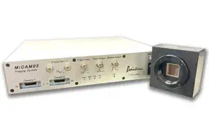
MiCAM03-N256 is a high-speed imaging system that captures and visualizes small changes in fluorescence intensity from biological samples stained with fluorescent probes, such as voltage sensitive dyes and calcium dyes.

Spatial Resolution : 

128x128 - 256x256 pixles
(32x32 pixels - 256x256 pixles with option)

Maximum Frame Rate : 

1,000fps
(20,000 fps available with option)

Up to 2 camera heads can be used with completely synchronization.

View More Details